One of the things that I didn’t realise until I started blogging was how interesting I would find the data collected on who actually reads my blog, where they’ve come from, and what they were looking for. As I expected based on the content I’ve published so far, many of my visitors have been looking for information on the Bing Maps tile system, on WMS servers, SQL Server spatial reference systems, and on terrain and elevation information. I hope that some of them have found some helpful information… However, last month, for example, I was also fascinated to find a number of people had found my site having searched for “Alastair Aitchison professional CV” – who are you? what were you looking for?!
Anyway, reading through my search engine referrals, another big area that people seem to be looking for information on is about using Ordnance Survey data in SQL Server. I have posted about the Ordnance Survey before, and about spatial data in SQL Server, but not specifically about the two together, so those people have probably been left disappointed. This post is an attempt to rectify the situation…
The Ordnance Survey, if you don’t know, is the national mapping agency of Great Britain, and it is the source of most of the high-quality mapping information in the country. For a long time, however, their data was tightly-controlled, and not affordable to use unless you were a large organisation capable of paying a corporate licence. This was hugely frustrating for small or charitable organisations trying to make use of spatial information.
Now, ex-Prime Minister Gordon Brown didn’t do much for the UK, but it is largely thanks to him that in the last year the situation has changed. The story goes that, at some formal dinner or other, Gordon Brown ended up having a conversation with Sir Tim Berners-Lee. The prime minister asked what the government should do to make better use of the internet, to which Berners-Lee replied “Put all the government’s data online”. It’s not happened overnight, but there have been some great steps taken towards increasing public access to UK government data, including crime information, census and demographic information, and spatial information from the Ordnance Survey. So here’s a step-by-step guide as to how to load that data.
Get Some OS Data
First, acquire the data from the Ordnance Survey Open Data website. There are several “products” to choose from. The ones I find most interesting are:
-
- Strategi, Meridian2, OS VectorMap District – vector polygon, polyline, and point features of e.g. administrative boundaries, developed land use areas, woodland, roads, rivers and coastline, at small- medium- and high- scale respectively.
- Code-Point Open – locates every postcode unit, and maps to corresponding coordinates / health authority / county etc.
- 1:50,000 Scale Gazetteer – as the name says, a gazetteer of placenames and locations
Note that the Ordnance Survey have not made all their data freely-available – if you want the really high-quality datasets (such as OS Mastermap), you’ll still have to pay for it, but OpenData gives you a good start. Even though the OpenData products are of limited resolution (equivalent to, say, the 1:50,000 Landranger series of maps), they are of good quality – better quality data than, say the equivalent TIGER data in the U.S – and they are much better than having no free data at all, which was the case 12 months ago…
Prepare the Data
Most OS datasets are provided in ESRI shapefile format. If you’re using one of the smaller scale datasets (e.g. Strategi or Meridian2), each feature layer (i.e. roads, rivers, railways) will come in its own shapefile. You’ll probably want to keep each layer in its table in the database, so this is fine.
However, if you want to load the larger scale OS VectorMap data you’ll find that it is split up into smaller files, each one labelled with the appropriate 100km x 100km grid square reference (e.g. TQ, TL, NT…). Then, within the download of each of these grid squares, there is a subdirectory for each 10km x 10km subsquare. So within the TQ directory there will be folders labelled TQ00, TQ01, TQ02, … , TQ99. Each of these subfolders follows exactly the same structure – containing one shapefile for each of the feature layers within that square. So, if you want to load the features of a complete 100km x 100km square of data in one go, you first need to merge the shapefiles in all of the subdirectories together. You can do so using OGR2OGR from the command line prompt as in the following script:
for /R %f in (*.shp) do (
if not exist %~nf.shp (
ogr2ogr -f “ESRI Shapefile” “%~nf.shp” “%f”
)
else (
ogr2ogr -f “ESRI Shapefile” -update -append “%~nf.shp” “%f”
)
)
This will look for all shapefiles in all subdirectories of the directory in which the script is run – if a file of the same name (e.g. AdministrativeBoundary.shp) has been found in another subdirectory already, they will be merged together, if not, a new file will be created. Resulting merged files will be created in the current directory. (This was adapted from a script by Darren Cope)
Load the Data
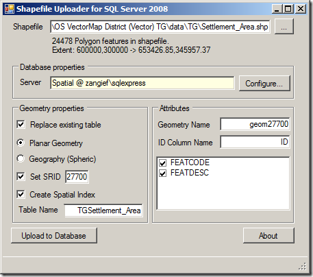
Having prepared the shapefiles, you can load them into SQL Server using a tool of your choice…. if you don’t want to splash out a commercial licence for Safe FME then I recommend Shape2SQL – you can use it to load shapefiles to SQL Server either via the GUI interface or via the commandline as described here.
Ordnance Survey data is defined using the National Grid of Great Britain, so always make sure that you load your data into a column of the geometry datatype, using SRID 27700.

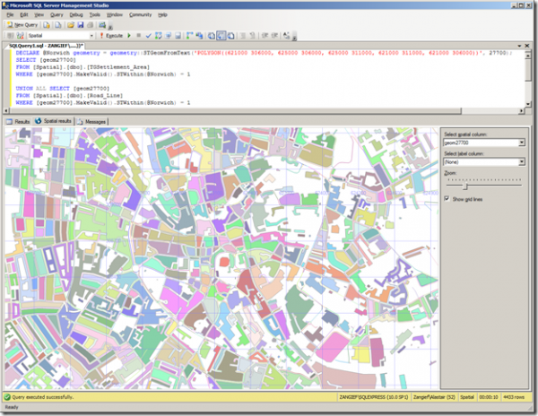
And that’s all there is to it! Here’s the data loaded from combined table of the OS Vector Map settlement_area and road_line shapefiles, showing the buildings and roads of the city centre of Norwich (still beautiful even when viewed in the pastel shades of SQL Server Management Studio):


