Flood Simulation HowTo

In his novel Book of Dave‘, Will Self imagines a world in the future where sea levels have risen over a 100m.

This destroys civilization as we know it but leaves London skyscrapers still standing half underwater in the sea – the remaining humans who live on ‘Ham’ (an island created from the rising sea surrounding the high ground of Hampstead Heath, London) climb one of these which they call ‘Central Stack’ to capture seagulls. As the book has a map of Ham in the front I played around in Google Earth to see how accurate the boundary of the island actually was, as it happens, Will’s imaginary island is what would really occur if sea level rose that far.

I realised the technique I used (one a teacher pointed out to me at a training session a while back) could be used in a lesson to visualize rising sea levels or ancient ice sheets. If you draw a polygon and give it an altitude that is about ground level the sheet created will disappear below the ground where the land is higher but be visible where the land is lower. Here’s how to create a series of these sheets in a folder so you can show a sequence of increasing sea levels :

  1. Click the Temporary Places folder in the Places column (it will get a background) then right click > Add > Folder. Add a name in the dialogue box and tick the ‘Show contents as options’ box. You’ll see why in a moment.
  2. Navigate to a location you want to ‘flood’ in the main screen. Right click the folder you’ve just created > Add > Polygon. Move the dialogue screen that opened out of the way (I move it to the bottom of the screen) and click the 4 corners of a square. Make it less than 10 miles across otherwise wierd things happen to the layer because of the curvature of the earth (I think, see note below)
  3. Drag the dialogue box back into view and under the ‘Style, Color’ using the controls titled ‘Area’ select an appropriate color for the square (blue for sea level rise, white for an ice sheet?) also select an opacity of 30% or so.
  4. Under the Altitude tab choose an altitude of 100m and then select ‘Relative to Ground’ in the pull down menu. This will raise your colored square 100m above the ground.
  5. Name your square something sensible but with a ‘100’ in it (e.g. “London 100m”) then click OK.
  6. Now right click the element you created in the Places column and select copy. Right click the copy >Properties > Altitude and change the altitude to 200m. Change the name to replace 100 with 200 and click OK.
  7. You should now have 2 sheets, one at 100m altitude and one at 200m. Clicking in the circles turns one on and the other one off automatically.
  8. Experiment with altitudes that works for your chosen location, copy and paste more sheets if necessary by repeating step [6] – within the folder you created only one sheet will be visible at any one time.
  9. Right click the folder and select ‘Save As’ to save and send to someone else.
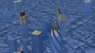
3D Buildings: It’s a lot of fun to turn on the 3D buildings layer whilst you have sheets visible in the layers column, as in the screeen shot the layers will show how deep buildings would be sunk in the sea – not sure if any of those in the screen shot are Central Stack.
Absolute Heights: Experimenting with the levels, the sheet behaves oddly, it doesn’t meet the land at the height you would expect. I’m not sure why this is but it may do with the curvature of the earth (in the middle of a big square the earth will protude through a level sheet even though there is no topography). If anyone has a definitive answer I’d like to know.

Surface Flicker: If you zoom into the layers from a distance you may see line of where land meets sheet flicker and change. This is because GEarth creates the view of the earth you see by taking the satellite images and draping them over a set of ‘posts’ it builds rather like a marquee tent. If you view the ground from a higher altitude GEarth uses fewer posts so the surface changes as you zoom in and out. There is a way around this but its fiddly, I’ll post about it if anyone’s interested.

London 3D Project

Jack recently contacted me to let me know about the “London 3D Project”, which I wasn’t previously aware of. They’re a group of users that want to see more 3D buildings in London and rather than complain about it, they’re getting to work! Since they started work in October, the team has constructed well over 100 models, and roughly 80 of them have shown up in Google Earth.

They’re making a point to try to tackle a lot of the “boring” buildings that people otherwise might not model. For example, there are over 200 models of “Big Ben” in the 3D Warehouse, and most of the popular buildings in town have multiple models available. Their effort is focused on filling out the city with all of the models they can find, not just famous buildings.

To learn more about the project, you can visit their website at www.london3dproject.mfbiz.com.

You can also check out some of their models in the 3D Warehouse.

A project like this is also a great way to explore a city. Jack mentioned that they’ve come across a variety of interesting architecture and some buildings that they didn’t even know existed. Not only have they discovered these buildings now, but they’re sharing them with the rest of the community. Great work guys!

London Twitter Network Map

Fabian Neuhaus author of Urban Tick here at the Centre for Advanced Spatial Analysis, University College London has kindly agreed to write a guest post on the London Twitter network, the zoomable version embedded below is particularly notable:

Following up from the New City Landscape maps, where we mapped tweet densities in urban areas around the world, we have now started to look into the socia network aspects of this data set. As a complementary graph to the map the network illustrates how the twitter users are connected through their activities and usage of the platform.

LND-NCL_NWgraph_s
Graph by urbanTick / The London NCL Social Network graph of twitter users. The dataset is defined as geolocated tweets collected over the period of one week in the urban area of London set to a 30 km radius. Click on the image for a larger version on flickr or see the interactive zoomable version HERE.

The network is built from nodes and edges, were the nodes are the twitter users active during the time period of message collection back in May 2010. The edges visualise the connections between these users. From the messages sent connections are established based on activity and interaction. In reality these are the @ messages that are directed at one or more particular user. The second indicator of a connection are the RT messages, the message that have been retweeted by followers of the creator of the initial message.

LND-NCL_NWgraph-04
Graph by urbanTick / Zoom of the London NCL Social Network graph of twitter users. The dataset is defined as geolocated tweets collected over the period of one week in the urban area of London set to a 30 km radius. Click for a larger version on flickr.

Using these two methods the network graph is established as a directed network, meaning that the connection between the nodes has a direction since a message originates from a sender being delivered to a receiver.

The resulting network is built from a total of 17618 nodes and 26445 edges. In the case of this London twitter network not everyone is connected to everyone and about 5400 subnetworks were identified. Furthermore via the colouring the modularity of the network is visualised. Each subgroups has a unique colour shading indicating groups with tighter connections.

London NCL Social Network

Graph by urbanTick using the GMap Image Cutter / London NCL Socia Network – Use the Google Maps style zoom function in the top left corner to zoom into the map and explore it in detail. Click HERE for a full screen view.

The sizing of the nodes is derived from the number of connections this particular node has for both incoming and outgoing edges.

For the comparison of the networks we are currently working on graphing out the whole range of NCL across the world in order to establish a analysis parameter set. We’ll keep you posted about the progress here.

To compare it, the geolocated London New City Landscape map. It is important to keep in mind that the graphs are not spatially representative as compared to the NCL maps which are properly geolocated.

london_contourColour_2
Image by urbanTick using the GMap Image Cutter / London New City Landscape Click HERE for a full screen view.


Post by Fabian Neuhaus, Urban Tick.